PML 10. Normalizing Flows (for Simulation-Based Inference)
Probabilistic Machine Learning Reading Group
Roi Naveiro
March 25, 2026
CUNEF Universidad
A Motivating Example
- Geostationary Earth Orbit (GEO) is a circular orbit about 36,000 km above the equator.
- The orbital period is one day.
- The satellite appears approximately fixed over one longitude on Earth.
- This makes GEO valuable for continuous communication, broadcasting, and weather monitoring.
A Two-Body World
The satellite would satisfy
\ddot{\mathbf r}(t) = -\frac{\mu}{\|\mathbf r(t)\|^3}\mathbf r(t).
- Here \mu is Earth’s gravitational parameter.
- In this simplified world, the orbit is fully determined by the initial position and velocity.
Placing A Satellite In GEO
Then, to place a satellite in GEO, we would simply:
- choose the GEO radius,
- give it the correct tangential velocity,
- let the two-body force do the rest.
The Ideal GEO Orbit
In that case, the ideal satellite orbit would satisfy
\mathbf{r}^*(t)= \begin{bmatrix} a\cos(\lambda_0+\omega t)\\ a\sin(\lambda_0+\omega t)\\ 0 \end{bmatrix}, \qquad \omega=\sqrt{\frac{\mu}{a^3}}.
with corresponding target velocity \mathbf{v}^*(t).
Real GEO Satellites Drift
The dynamics are affected by more than central gravity:
\mathbf a(\mathbf r(t),t) \simeq \mathbf a_{\mathrm{grav}} + \mathbf a_{J_2} + \mathbf a_{3B} + \mathbf a_{R}.
- \mathbf a_{J_2}: Earth oblateness
- \mathbf a_{3B}: Sun and Moon
- \mathbf a_R: solar radiation pressure
Why We Need Control
So we need a controller that applies corrective acceleration \mathbf a_C to keep the satellite near the target orbit.
\mathbf a(\mathbf s(t),t,\boldsymbol\phi) \simeq \mathbf a_{\mathrm{grav}} + \mathbf a_{J_2} + \mathbf a_{3B} + \mathbf a_{R} + \textcolor{red}{\mathbf a_{C}(\mathbf s(t),t,\boldsymbol\phi)}.
A Controller: PD Station-Keeping
\mathbf s(t)= \begin{bmatrix} \mathbf r(t)\\ \mathbf v(t) \end{bmatrix} \in\mathbb R^6.
A Controller: PD Station-Keeping
Let
\Delta \mathbf r_t=\mathbf r(t)-\mathbf r^*(t), \qquad \Delta \mathbf v_t=\mathbf v(t)-\mathbf v^*(t).
Then a simple proportional-derivative policy is
\mathbf a_C^{PD}(\mathbf r_t,t,\boldsymbol\phi) = -K_p\,\Delta \mathbf r_t -K_d\,\Delta \mathbf v_t, \qquad \boldsymbol\phi=(K_p,K_d).
- K_p: how strongly we react to position error
- K_d: how strongly we damp velocity error
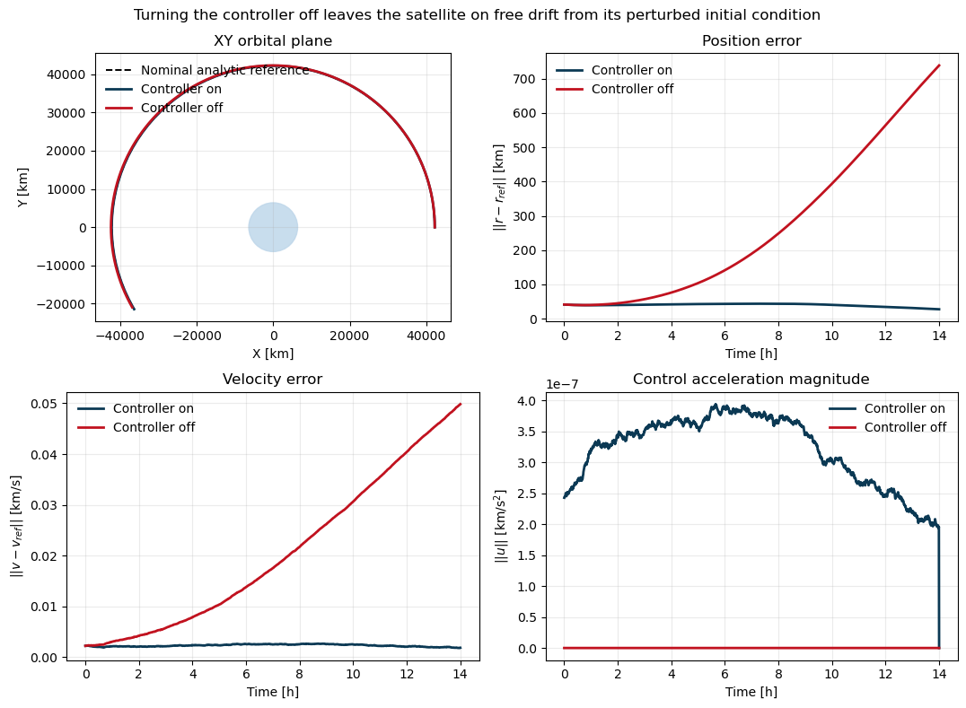
The Effect of the Controller
The Inference Problem
Suppose an observer collects a trajectory over an observation window:
\mathcal D=\{ \mathbf s(t_j),t_j\}_{j=1}^J,
where
\mathbf s(t_j)= \big[x(t_j),y(t_j),z(t_j),\dot x(t_j),\dot y(t_j),\dot z(t_j)\big]^\top.
The Inference Problem
Can we infer the controller parameters \boldsymbol\phi from the observed orbit?
A Bayesian Approach
The observer models the satellite with the SDE
d\mathbf s(t) = \mathbf f(\mathbf s(t),t,\boldsymbol\phi)\,dt + \mathbf G\,d\mathbf W(t),
where
\mathbf f(\mathbf s(t),t,\boldsymbol\phi) = \begin{bmatrix} \mathbf v(t)\\ \mathbf a(\mathbf s(t),t,\boldsymbol\phi) \end{bmatrix}.
The Model Components
The acceleration is
\mathbf a(\mathbf s(t),t,\boldsymbol\phi) = \mathbf a_{\mathrm{grav}} + \mathbf a_{J_2} + \mathbf a_{3B} + \mathbf a_R + \mathbf a_C(\mathbf s(t),t,\boldsymbol\phi).
- \mathbf a_{\mathrm{grav}}+\mathbf a_{J_2}+\mathbf a_{3B}+\mathbf a_R: known physics
- \mathbf a_C(\mathbf s(t),t,\boldsymbol\phi): controller action
- Unknown parameters: \boldsymbol\phi=(K_p,K_d)
The Bayesian Model
Once \mathcal D is observed, Bayesian inference targets
p(\boldsymbol\phi\mid \mathcal D) \propto p(\mathcal D\mid \boldsymbol\phi)\,p(\boldsymbol\phi).
This Likelihood is very Hard!
- The dynamics are nonlinear.
- The transition density of the SDE is not available in closed form in general.
We do not have an explicit formula for the likelihood of the observed path:
p\big(\mathbf s(t_1),\mathbf s(t_2),\ldots,\mathbf s(t_J)\mid \boldsymbol\phi\big).
But We Can Simulate from the SDE!
- Even if the likelihood is unavailable, we can simulate trajectories from the model.
\mathbf s(t) \sim p(\cdot\mid \boldsymbol\phi).
Numerically solving the SDE, we can generate as many trajectories as we want for any given \boldsymbol\phi.
Keep only the observed times.
How Do We Do Bayesian Inference With Only A Simulator?
SBI notation:
\theta := \boldsymbol\phi, \qquad x := \big(\mathbf s(t_1),\ldots,\mathbf s(t_J)\big).
How Do We Do Bayesian Inference With Only A Simulator?
We can simulate from the prior and evaluate its density: \theta\sim p(\theta),
We can simulate from the likelihood but not evaluate its density: x\sim p(x\mid \theta).
The Goal
- Given an observed trajectory x_o, we want to learn the posterior
p(\theta\mid x_o) \propto p(x_o\mid \theta)\,p(\theta).
An Idea
- Imagine a family of conditional densities q_\phi(\theta\mid x) with three key properties:
- Flexible enough to approximate complicated posteriors p(\theta\mid x)
- Easy to evaluate \log q_\phi(\theta_i\mid x_i)
- Easy to sample from q_\phi(\theta\mid x)
How Would We Find the Best q_\phi?
- Generate many simulated pairs
\theta_i\sim p(\theta), \qquad x_i\sim p(x\mid \theta_i).
- Then fit \phi by minimizing \hat\phi = \arg\min_\phi \frac{1}{N}\sum_{i=1}^N \big[-\log q_\phi(\theta_i\mid x_i)\big].
Equivalently, in the limit
\hat\phi \approx \arg\min_\phi \mathbb E_{p(\theta,x)}[-\log q_\phi(\theta\mid x)].
- Note that, to evaluate the objective, we only need to evaluate q_\phi(\theta\mid x)!
Why Does This Recover The Posterior?
- The loss is an average KL divergence plus a constant:
\mathbb E_{p(x)} \Big[ \mathrm{KL}\!\big(p(\theta\mid x)\,\|\,q_\phi(\theta\mid x)\big) \Big] + C
where C does not depend on \phi.
- Therefore the optimum is reached when
q_\phi(\theta\mid x)\approx p(\theta\mid x).
After Training
- We only need to plug in the observed trajectory:
q_\phi(\theta\mid x_o).
- This gives a learned approximation to the posterior.
- That is the basic idea behind neural posterior estimation.
Why One Round Is Often Wasteful
- In principle, q_\phi(\theta\mid x) is being trained for many possible data sets x.
- But in our problem we only care about one data set: x_o.
- So most simulations are useful only if they are informative near x_o.
SNPE Uses Multiple Rounds
Recall that for training we need pairs (\theta_i,x_i) where \theta_i\sim p(\theta) and x_i\sim p(x\mid \theta_i).
Round 1 samples from the prior: \tilde p_1(\theta)=p(\theta).
Train a first approximation q_{\phi_1}(\theta\mid x).
Later Rounds Focus Near x_o
Use the current approximation at the observed data as a proposal: \tilde p_r(\theta)\approx q_{\phi_{r-1}}(\theta\mid x_o).
Then simulate new pairs \theta_i\sim \tilde p_r(\theta), \qquad x_i\sim p(x\mid \theta_i),
The Missing Ingredient
We need a model q_\phi(\theta\mid x) that
Sample easily (for later rounds): \theta \sim q_\phi(\theta\mid x)
Evaluate densities exactly (for training each round): \log q_\phi(\theta\mid x)
Be flexible enough to learn complicated posteriors.
Enter Normalizing Flows
Say we want to model a complex density p_x(x) on \mathbb R^D.
Start from a simple base density u \sim p_u(u), e.g. a standard Gaussian.
Apply an invertible map f:\mathbb R^D\to\mathbb R^D.
The transformed variable x=f(u) now has a richer density.
Easy to Sample
u\sim p_u(u), \qquad x=f(u).
- Sampling only requires drawing from the base and applying the map.
Easy to Evaluate
If: x = f(u), \qquad g(x)=f^{-1}(x)=u.
Then
p_x(x) = p_u(u)\left|\det J(f)(u)\right|^{-1}.
Easy to Evaluate
Therefore
\log p_x(x)=\log p_u(u)-\log\left|\det J(f)(u)\right|.
- So density evaluation is efficient if g=f^{-1} and \det J(g) are easy to compute.
Flexible by Composition
If f_1,\dots,f_N are invertible maps then f = f_N \circ \cdots \circ f_1,
is also invertible and:
\log \left|\det J(g)(x)\right| = \sum_{i=1}^N \log \left|\det J(g_i)(u_i)\right|.
- Each layer contributes one simple deformation.
- Stacking many such layers yields a highly expressive density.
How Flows Are Trained For Density Estimation
- Given data \{x_n\}_{n=1}^N, maximize exact log likelihood:
\max_\omega \sum_{n=1}^N \log p_\omega(x_n).
How Flows Are Trained For Density Estimation
- For a flow,
\log p_\omega(x) = \log p_u\!\big(f_\omega^{-1}(x)\big) + \log\left|\det J\!\big(f_\omega^{-1}\big)(x)\right|.
How Flows Are Trained For Density Estimation
We can learn the parameters \omega by gradient ascent on the exact log likelihood, provided we can:
- efficiently evaluate the inverse u=f_\omega^{-1}(x),
- efficiently evaluate the Jacobian determinant,
And everything must remain differentiable in \omega.
For sampling, in addtion to the above, we also need to:
- efficiently evaluate the forward map x=f_\omega(u).
Types of Flows
How do we propose normalizing flows that satisfy the above properties?
f = f_N \circ \cdots \circ f_1,
Some Important Flow Building Blocks
- Elementwise
- Coupling
- MAF
Elementwise Flows
- Apply a (parametric) scalar bijection to each coordinate:
f(u)=\big(h(u_1),\dots,h(u_D)\big).
- The functions h are the source of flexibility here, and each one must be invertible.
Why Elementwise Is Efficient
- The Jacobian is diagonal, so
\log |\det J(f)(u)| = \sum_{i=1}^D \log \left|h_i'(u_i)\right|.
- Log determinant: D scalar derivatives, so O(D)
- Inverse x \mapsto u: D scalar inversions, so O(D)
- Forward map u \mapsto x: D scalar evaluations, so O(D)
- Limitation: no dependence across dimensions
Coupling Flows
Partition the input as u=(u_A,u_B) and define
\begin{aligned} x_A &= \hat f\big(u_A;\eta(u_B)\big) \\ x_B &= u_B. \end{aligned}
- The conditioner \eta(u_B) can be any neural network.
- It does not need to be invertible.
Coupling Inverse
u_B = x_B, \qquad u_A = \hat f^{-1}\big(x_A;\eta(x_B)\big).
- First recover the unchanged block
- Evaluate the conditioner once on the known block: \eta(x_B)
- Then invert only the transformed coordinates
Why Coupling Is Efficient
- Its Jacobian is block triangular:
J(f)= \begin{bmatrix} J(\hat f) & * \\ 0 & I \end{bmatrix}
so
\det J(f)=\det J(\hat f).
Why Coupling Is Efficient
If C_\eta denotes the cost of one conditioner-network evaluation, and |A| is the size of the transformed block, then:
- Inverse x \mapsto u: C_\eta + O(|A|)
- Log determinant: O(|A|), only block A contributes
- Forward map u \mapsto x: C_\eta + O(|A|)
From Coupling To Autoregression
- In coupling, one block conditions another block.
- In the extreme case, each coordinate can depend on all previous ones.
Autoregressive Flows
Define
x_i = h\big(u_i;\eta_i(x_{1:i-1})\big), \qquad i=1,\dots,D.
Then the Jacobian is triangular:
\frac{\partial x_i}{\partial u_j}=0 \qquad \text{for } j>i,
Why The Mask?
- A naive approach would use D different neural networks, one for each conditioner \eta_i.
- MAF uses one shared network instead.
- This network takes x as input and outputs all conditioner values \eta_i at once.
- The mask zeroes connections from x_j to \eta_i whenever j\geq i so \eta_i still depends only on x_{1:i-1}, but parameters are shared.
Masked Autoregressive Flows
u_i = h^{-1}\big(x_i;\eta_i(x_{1:i-1})\big), \qquad i=1,\dots,D.
- Inverse x \mapsto u:
- one masked-network evaluation
- then D scalar inversions, usually closed form
- total: C_\eta + O(D)
Masked Autoregressive Flows
- Log determinant:
\log \left|\det J\!\big(f^{-1}\big)(x)\right| = \sum_{i=1}^D \log \left| \frac{\partial}{\partial x_i} h^{-1}\big(x_i;\eta_i(x_{1:i-1})\big) \right|.
- Cost C_\eta + O(D).
Masked Autoregressive Flows
x_i = h\big(u_i;\eta_i(x_{1:i-1})\big), \qquad i=1,\dots,D.
- Forward map / sampling u \mapsto x:
- sequential, because x_i depends on x_{1:i-1}
- after generating x_1, we can compute x_2, then x_3, etc.
- total: roughly D\,C_\eta + O(D)
Illustration
- A very simple visual comparison is in:
Notebook 1
Back to the Satellite Problem
- The full SBI example is in:
Notebook 2 satellite_sbi/notebooks/minimal_sbi_satellite_joint_demo.ipynb
Conclusion
- Simulation-based inference reduces the problem to learning p(\theta \mid x) from simulations.
- Normalizing flows are useful because they keep exact densities and efficient sampling.